Humans developed the extraordinary capability of verbal communication. We can convey our thoughts and ideas in written or spoken word. This is a process of transferring information from one entity to another, much like computers on the internet. During every transfer of information, errors can occur, corrupting the message. Therefore methods of detecting errors are needed. In machine communications, this is often done with checksums. These error correction measures lead to that not all transmitted data contains new information.
Information
The meaning of the word information differs from everyday usage in the context of information theory. When one speaks of information, one usually means meaning. Roughly speaking, the information is a measure of freedom in choosing a message. In connection with language, we are interested in the information density and redundancy of our language. We want to know how much information a letter provides.
Entropy
We require a function $H(p_1, \dots, p_n)$ with the following properties:
- $H(p_1, \dots, p_n)$ is continous for all $p_i$.
- If $p_i=\frac{1}{n}$ then $H(\frac{1}{n}, \dots, \frac{1}{n}) < H(\frac{1}{n+1}, \dots, \frac{1}{n+1})$
It can be shown that these requirements uniquely define a function
$H(p_1, \dots, p_n) = – \sum_i p_i \log p_i$
which is called entropy.
Calculation of the entropy of languages
The Entropy of n-grams is defined as the following:
$H_n = – \sum_i p(b_i^n) \log_2 p(b_i^n)$
The information content of a letter results from the difference
$F_n = H_{n+1} – H_n$
of the entropy of the (n+1)-grams and the n-grams. $F_n$ is called conditional entropy. From the requirements on the entropy function $H$ follows that $F_n$ has a positive limit $E$. This is the law of Shannon:
$E = \lim_{n \rightarrow \infty} F_n$
Choosing $\log_2$ allows one to interpret $E$ as the number of Bits or yes-no decisions, that are necessary to determine one letter.
To calculate $F_n$ the relative probabilities $p(b_i^n)$ must be determined. This is done by choosing a sufficiently large text body and counting the occurrence (frequency) of every n-gram inside the text.
Redundancy and relative entropy
Now it is not only of interest to determine the information of a letter, but also the percentage of our language that contains no information. Entropy is maximized when all occurring n-grams are equally probable. In the case of the Latin alphabet, including spaces, $p_n = \frac{1}{27^n}$ applies and for the maximum entropy $M_n$ one verifies:
$M_n = – \log_2 p_n$
Now we can give a measure for the information-carrying fraction of a language as:
$G_n = \frac{H_n}{M_n}$
This is equivalent to the maximum possible compression in the given alphabet. Therefore it is possible to determine the entropy of the language, or rather an upper limit, by compressing text. The proportion of a text without information, the redundancy, is then consequently:
$R_n = 1 – G_n$
Implementation
To compare different languages a good data source is needed. Wikipedia is ideal for this. Availability in many different languages, and clear and liberal licensing make Wikipedia the ideal data source. The text is of high quality and one does not have to deal with erroneous scans.
Three C++ programs were written to analyze the text of wikipedia.
The entropy of nine different European languages was examined, and the investigation was limited to languages with the Latin alphabet. Therefore a certain homogeneity of the results is to be expected. The following table shows the used text corpora sorted by size.
| EN | DE | FR | ES | IT | SV | NL | PL | PT | |
| Size [GB] | 13 | 6,1 | 5,5 | 3,8 | 3,2 | 2,4 | 1,8 | 1,8 | 1,7 |
| N. Articles $\times 10^6$ | 5,8 | 2,3 | 2 | 1,5 | 1,5 | 3,7 | 2 | 1,3 | 1 |
Results
The results of the calculated conditional entropies can be seen in the next figure:
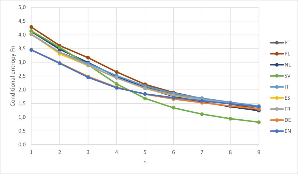
It can be seen that all analyzed languages seem to converge to a value near $1$. The only exception seems to be Swedish with significantly lower entropy. Whether this is an actual feature of the Swedish language or has other causes is not clear. A possible reason is that the Swedish Wikipedia is the second largest by number of articles, but the absolute text size is quite small. It is conceivable that the result will be falsified if the entries are structured in the same way. Just think of the always similar article beginning of personal entries. This explanation is also supported by the fact that the effect would only become noticeable at higher n-gram orders, as is the case. It is also interesting that German and English show an almost identical progression. The inhomogeneous frequency distribution of the letters (1-gram) of these two languages is reflected in a low entropy at $n=1$. The maximum entropy for the 27-character alphabet is $M_1 = \log_2 27 \approx 4.75$. Polish comes closest to this value.
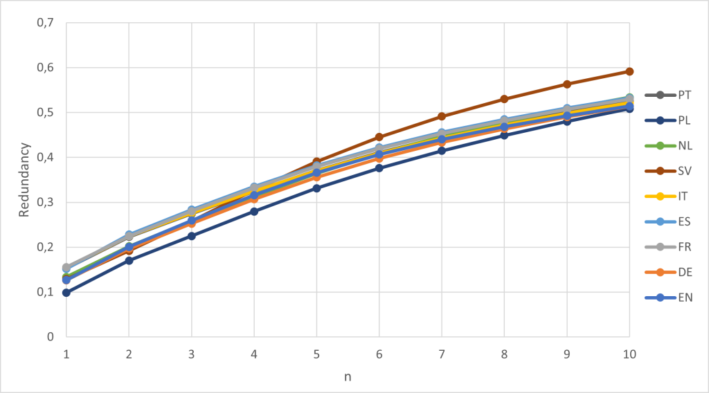
The redundancy for the nine languages is plotted in Fig. 2. The redundancy is just over 50% for all languages except Swedish. This means that around half of the letters in a text do not contain any information. As Shannon reasons in his original paper, this is why it is possible to play crossword puzzles.
Zipf’s law and $\frac{1}{f}$-noise.
Zipf’s law was first introduced by G.K. Zipf in the 1930s and states the following: If the words are arranged according to their frequency then the relative frequency $f(r)$ of a word is inversely proportional to its rank $r$.
$f(r) = \frac{a}{r^\gamma}$
It is roughly $a\approx 0.1$ and $\gamma \approx 1$.
The 1/f behavior is clearly shown if the number of different n-grams is plotted against the n-gram frequency (number of occurrences in a text) in a double logarithmic manner. In Fig. 3 this can be seen for the trigrams of the German language.
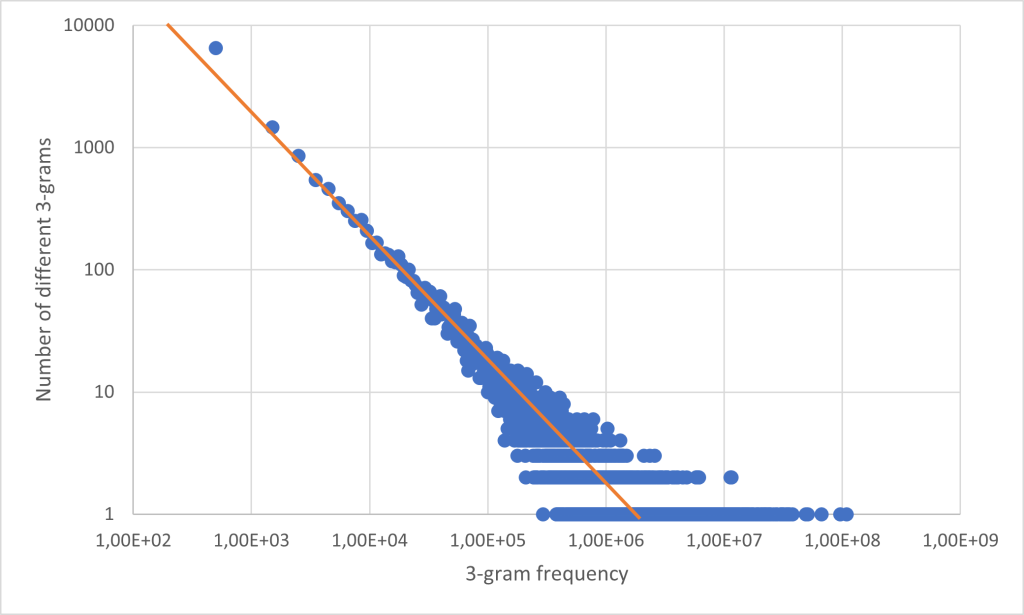
The plot can be understood as follows: The point on the far left says that there are about 9000 different tri-grams that occur less than 1000 times in the text. To create the histogram, the tri-gram frequency was divided into bins with a width of 1000.
Zipf’s law can then be obtained from this data by assigning a rank to the trigrams according to their frequency and plotting the relative frequency of the same. The result can be seen in Fig. 4.
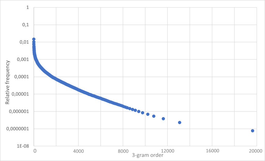
Zipf’s law originally referres to single words. But as can be seen, the tri-grams are also subject to this behavior. However, the true nature of the $\frac{1}{f}$ behavior is better represented in the representation of the trigram frequencies.
Conclusion
In the context of this work, only languages with the Latin alphabet were examined. It would be very interesting to study languages with other alphabets such as Cyrillic languages. Furthermore, it might be worth examining the statistics of the planned languages Esperanto and Interlingua. The process of language formation is a Markov chain of extremely large order. The probability of going from one n-gram state to another depends heavily on the past states. The transition probabilities of the n-grams are contained in the frequency table of the 2n-grams. Without much effort one could write a program that calculates the transition matrix from the frequency tables. Using the transition matrices for large $n$, one could examine the statistical process of language formation for ergodicity.
The C++ programs written to analyze the text corporas together with some example data can be found here.
A more detailed analysis can be found in my german essay as well in a poster i made.
References
- C.E. Shannon, Prediction and Entropy of Printed English, Bell System Technical Journal 30 379-423 (1951)
- L.B. Levitin, Z. Reingold, Entropy of Natural Languages: Theory and Experiment, Chaos Solitons & Fractals 4, 709-743 (1994)
- C.E. Shannon, A Mathematical Theory of Communication, Bell System Technical Journal 27 379-423, 623-656 (1948)
- G. K. Zipf, The Psycho-biology of Language: An Introduction to Dynamic Philology. Houghton Mifflin Company (1935)
- W. H. Press, Flicker Noises in Astronomy and Elsewhere, Comments Astrophys. 7 103-119 (1978)
- S. Roman, Coding and Information Theory, Springer (1992)