Numerical solution of the Gross-Pitaevskii-Equation

When matter is cooled down to extreme temperatures near absolute zero strange but fascinating things happen. There are two fundamental groups of particles, Bosons, and Fermions which behave differently at $T=0\text{K}$. While Bosons will all occupy the same quantum mechanical ground-state, two Fermions will never occupy the same quantum state. The phenomenon for Bosons to all condense into the lowest ground-state is called Bose-Einstein-Condensation, BEC for short. The equation which describes the behavior of Bosons in this quantum state is the Gross-Pitaevskii-Equation, for short GPE. It is named after its two independent discoverers Lev Pitaevskii and Eugene P. Gross.

There is the time independent

$\left( -\frac{\hbar^2 \Delta}{2m} + V(\boldsymbol{r}) + g \lvert \psi (\boldsymbol{r}) \rvert ^2 \right) \psi (\boldsymbol{r}) = \mu \psi (\boldsymbol{r})$

and time dependent GPE:

$i \hbar \frac{\partial}{\partial t} \Psi (\boldsymbol{r},t) = \left( – \frac{\hbar^2 \Delta}{2m} + V(\boldsymbol{r},t) + g \lvert \Psi (\boldsymbol{r},t) \rvert ^2 \right) \Psi (\boldsymbol{r},t)$

Except in a few limiting cases, there are no analytical solutions and the equations have to be solved numerically. Usually, the Crank-Nicolson method or the Fourier split-step method is used. The latter will be explained in this post. We will explain how the algorithm works with the Schrödinger equation and then how it can be applied to the GPE.

Fourier split step algorithm

The Schrödinger equation

$i\hbar \frac{\partial \Psi(\boldsymbol{r},t)}{\partial t} = -\frac{\hbar^2}{2m}
\Delta \Psi(\boldsymbol{r},t) + V(\boldsymbol{r}) \Psi(\boldsymbol{r},t)$

has, as long as $V(\boldsymbol{r})$ is time-independent, the time evolution operator

$U(\Delta_t) = e^{-\frac{i \Delta_t}{\hbar} (T+V)}$

with the kinetic energy $T = -\frac{\hbar^2}{2m} \Delta $ and time step $\Delta_t$. The time evolution of $\Psi(\boldsymbol{r},t)$ is then given as:

$\Psi(\boldsymbol{r},t + \Delta_t) = e^ {- \frac{i \Delta_t}{\hbar} (T + V)} \Psi(\boldsymbol{r},t)$

The algorithm is now based on the fact, that $V$ is diagonal in spatial and $T$ in momentum space. Because of modern FFT routines the transformation between both can be computed efficiantly. But $T$ and $V$ do not commute so $ e^ {- \frac{i \Delta_t}{\hbar} (T + V)} \neq e^ {- \frac{i \Delta_t}{\hbar} T} e^ {- \frac{i t}{\hbar} V} $. Nonetheless, it can be shown, that the approximation

$e^ {- \frac{i \Delta_t}{\hbar} (T + V)} \approx e^ {- \frac{i \Delta_t}{2\hbar} V} e^ {- \frac{i \Delta_t}{\hbar} T} e^ {- \frac{i \Delta_t}{2\hbar} V}$

is already quite good. With this a time evolution step can be computed as follows:

$\Psi(\boldsymbol{r},t + \Delta_t) \approx e^ {- \frac{i \Delta_t}{2\hbar} V(\boldsymbol{r})} \mathscr{F}^{-1} \{ e^ {- \frac{i \hbar \Delta_t}{2m} k^2} \mathscr{F} \{ e^ {- \frac{i \Delta_t}{2\hbar} V(\boldsymbol{r})} \Psi(\boldsymbol{r},t) \} \}$

Extension to the GPE

The FSSA was first developed for the time evolution of the linear Schrödinger equation. The more surprising is that, with the substitution

$V(\boldsymbol{r}) \rightarrow V(\boldsymbol{r}) + g |\Psi(\boldsymbol{r},t)|^2$

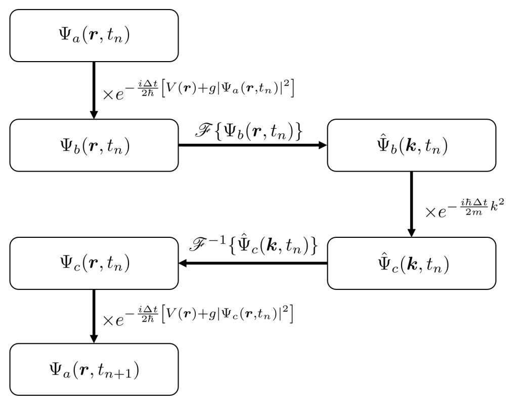
the FSSA can be applied to the GPE. In the following figure the numerical flow chart of the algorithm is shown:

Imaginary time evolution

The imaginary time evolution is a method for computing the ground state, given a suitable time evolution algorithm. It is based on the simple substitution:

$t \rightarrow -it$

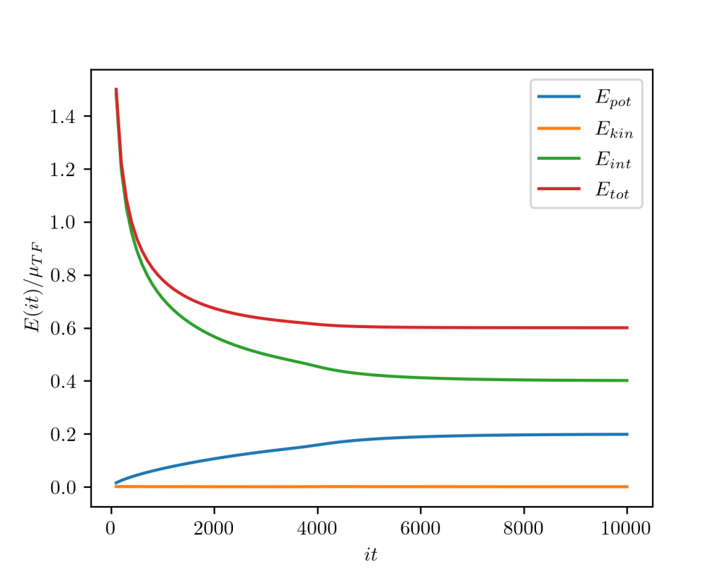
With the advent of sufficiently powerful computers in the 1960s, it became possible to calculate the ground states of the Schrödinger equation in this way. Since the GPE contains a non-linear term, it is initially unclear whether the method will also work with it. So are for example, the eigenstates of the nonlinear Hamiltonian generally not orthogonal to one another. Experience shows, however, that the method also delivers good results with the GPE. A suitable initial state $\Psi(\boldsymbol{r},0)$ is propagated in imaginary time. To judge whether the evolved state is close enough to the groundstate or not, the energy is calculated at every imaginary time step. If the energy difference between two steps is sufficiently small, the evolution is stopped. The follwing figure shows the typical behaviour of the different energy contributions during a imaginary time evolution:

It is very instructive to save the wavefunction at every imaginary time evolution step and make a movie from it. This has been done in the follwing animation, which shows the computation of the groundstate of a BEC produced in an optical dipole trap: